No-code model observability

With no-code integration, any Superwise user can now connect a model and define the model’s schema, and log production data via our UI with just an excel file.
With no-code integration, any Superwise user can now connect a model and define the model’s schema, and log production data via our UI with just an excel file.
Scaling up your model operations? in this blog we will offer some practical advice on how to build your MLOps roadmap
Learn how to integrate MLflow & Superwise, two powerful MLOps platforms that manage ML model training, monitoring, and logging
What keeps you up at night? If you’re an ML engineer or data scientist, then drift is most likely right up there on the top of the list. But drift in machine learning comes in many forms and variations. Concept drift, data drift, and model drift all pop up on this list, but even they only scratch the surface of much more nuanced problems. In this article, we’ll review all the types of drift and the nuances of each of them, as well as best practices to monitor, detect, investigate, and resolve drift in machine learning.
More posts in this series:
“The only constant in life is change” ( Heraclitus of Ephesus, ~500 BC)
Our world is constantly changing. And what’s true and obvious today may not be so tomorrow. This is undoubtedly on-point in the world of machine learning. The ultimate goal of machine learning models is to extract patterns from past data and use them to predict future behavior for unseen instances. These patterns, also referred to as ‘concepts,’ are fundamental to machine learning because they help classify data and recognize relationships between different variables.

When these relationships change in the real world–as they inevitably do–the patterns our model learned become invalid and can limit the model’s predictive power. This ‘model drift’ tends to happen when a model moves from development to a live production environment, when the data changes, or when situations in the real world change.
We tend to assume that a model will make correct predictions once it goes into production. After all, if we didn’t think so, we would continue to retrain the model until we felt it worked well enough to be deployed to the real world. However, most of us can attest to the fact that the real-world waits for no one, and that holds true for the data our models run on. Meaning that from day 1, the data that our models utilize to make predictions is already different from the data on which they trained. And depending on the degree of change, our models may suffer from model drift and model decay, unwanted bias, or even just being suboptimal given the type of drift we are faced with. Drift may signal that our results will worsen over time or show suboptimal performance in specific slices of data or populations.
What causes drift in ML? It can be anything from errors in data collection, changes in the way people behave, or even time gaps that alter what is considered a good prediction and what is not. An example of model drift could be an ML model whose algorithms help approve or reject loans for bank customers. In the past, most people requesting loans were between the ages of 32 and 40, with specific behavior profiles. But today, 80% of loan requests are from people under the age of 30. In this case, the model must be optimized for the new mix of data, or it will offer incorrect predictions when it comes to who is a good loan candidate.
As more and more machine learning models are deployed and used in live environments for real-world applications, model drift has become a major issue. In our digital and big data era, it’s unrealistic to expect data distributions to remain stable over a long period of time. This means drift is a top concern for data science teams scaling their use of ML. Let’s face it, the amount of time we spend maintaining model health is going up exponentially. It has definitely become a core—and painful—part of the day-to-day tasks for any team maintaining models in a live production environment.

Concept drift or model drift is sometimes used as a generic term to describe any changes in the statistical properties of the data. Mathematically, it indicates changes in the distribution P(y | X), which describes the relationship between the predictors and the target variables. The common formal definition for concept drift is: “a change in the joint probability distribution, i.e., Pt(X,y) ≠ Pt+(X,y).” It’s also referred to as ‘dataset shift.’ We can decompose the joint probability P(X,y) into smaller components to better understand what changes in these components can trigger concept drift:
Some researchers also distinguish between ‘real’ and ‘virtual’ concept drifts, where real concept drift refers to changes in P(y | X) and virtual concept drift refers to changes in P(X) or P(y) that don’t affect the decision boundaries or the posterior probabilities P(y | X). Although these ‘virtual’ changes appear to be less serious, they tend to be a side effect of the real ones. It’s hard to imagine a real-world application in which P(X) changes without impacting P(y | X).

Although researchers may need to distinguish between real and virtual drift, we need to monitor real-world applications for all types of drifts. Here’s why:
Drift in machine learning can occur for any number of reasons, but these causes generally fall into two main groups: bad training data and changing environments.
Bad training data that doesn’t accurately represent real-world situations is also known as unrepresentative training data:
Changing environments
The word ‘drift’ generally implies a gradual change over time. But these changes in data distribution over time can manifest in different shapes and sizes. Here are some of the different ways they take place based on transition speed:

These different patterns in which models drift bring us directly to the issue of detecting ML drift. Because drift in the wild takes different forms, different methods are needed to detect each. Take, for example, detecting seasonal model drift, which requires methods that rely on time series analysis; these know how to decompose seasonal aspects versus statistical process controls that are primarily used to detect sudden or outlier changes. There are a few common statistical measures used to calculate these drifts, and in the next post on the subject, we’ll dive into that as well.
As the ML industry and MLOps, in particular, become increasingly more mature, it’s essential to align the terminology among practitioners. Drift is a fundamental concept that needs to be understood by every ML practitioner. While general macro drift may occur occasionally, smaller local drifts on specific subpopulations or segments happen on a frequent basis and usually get by under the radar. While concept drift is often referred to as one major issue, as we saw in this post, it can be divided into many different types of drift in ML that happen for various reasons and may appear in different formats. Understanding all the possible patterns and types is an important step in detecting them efficiently and understanding how to deal with and fix their actual root cause.
Head over to the Superwise platform and get started with easy, customizable, scalable, and secure model observability for free with our community edition.
Request a demo and our team will show what Superwise can do for your ML and business.
Due to the increased usage of ML-based products within organizations, a new CI/CD like paradigm is on the rise. On top of testing your code, building a package, and continuously deploying it, we must now incorporate CT (continuous training) that can be stochastically triggered by events and data and not necessarily dependent on time-scheduled triggers.
The following post will show how fast and easy it is to set up a robust training-serving pipeline that will execute automatically based on production data and ongoing events. Notebook and repo included.
As the ML ecosystem grows, more and more companies are adopting and integrating ML-powered solutions for internal use and customer-facing products. However, as we all know, machine learning algorithms are a bit of a black box. While experimentations and development during the data science phase may look promising, when the time comes for your models to contend with the real world, many things can go wrong due to constantly evolving data profiles.
Machine learning-based software adds an extra layer of complexity to the traditional CI/CD pipeline, the reasons being:
Team skills
In an ML project, the team usually includes data scientists or ML researchers who focus on exploratory data analysis, model development, and experimentation. These members might not be experienced software engineers who can build production-class services.
Development
ML is experimental in nature. You should try different features, algorithms, modeling techniques, and parameter configurations to find what works best for the problem as quickly as possible. The challenge is tracking what worked and what didn’t and maintaining reproducibility while maximizing code reusability.
Testing
Testing an ML system is more involved than testing other software systems. In addition to typical unit and integration tests, you need data validation, trained model quality evaluation, and model validation.
Deployment
In ML systems, deployment isn’t as simple as deploying an offline-trained ML model as a prediction service. ML systems can require you to deploy a multi-step pipeline to automatically retrain and deploy the model. This pipeline adds complexity and requires you to automate steps that are manually done before deployment by data scientists to train and validate new models.
Production
ML models can have reduced performance not only due to suboptimal coding but also due to constantly evolving data profiles. In other words, models can decay in more ways than conventional software systems, and you need to consider this degradation. Therefore, you need to track summary statistics of your data and monitor the online performance of your model to send notifications or roll back when values deviate from your expectations.
MLOps: Continuous delivery and automation pipelines in machine learning, Google
In production, without the ability to observe, detect, and automatically fix unexpected behavior, an ML-infused product is on the highway to failure.
While tackling each of the points above can be a great topic for a book, our goal in this post is to demonstrate how we can achieve a robust training pipeline that will be triggered by training-serving data skew.
Prerequisites:
GCP Stack:
We will use the following GCP components:
Vertex pipeline (Kubeflow based) for the training-serving pipeline.
Vertex model & endpoint for serving our model to a production-like environment
Google storage – for storing the artifact, pipeline outputs, and our trained model before deployment
Google artifactory registry to store our custom predictor image
Google Cloud function – to simulate an HTTP webhook that will trigger a retraining pipeline
Assets:
Let’s go ahead and create a service user. This service user will be responsible for performing all the GCP operations from within the customized docker image. In the GCP navigation menu -> IAM -> service accounts -> create. After the service account has been created, generate a JSON key file. This key file will be stored later on inside the image, so keep it in a safe place for now (Google tutorial).
In a new terminal, set a new environment variable:
export GOOGLE_APPLICATION_CREDENTIALS=<path_to_key_file>
And run
gcloud init.
Authenticate your Google account and follow the instructions to set up the connection. From here on out, we can use gcloud and gsutil from the terminal to perform actions in GCP.
To enable all the GCP components mentioned above, run the following:
gcloud services enable compute.googleapis.com         \
                       containerregistry.googleapis.com  \
                       aiplatform.googleapis.com  \
                       cloudbuild.googleapis.com \
                       cloudfunctions.googleapis.com
“Operation “operations/acf.p2-<some unique id>” finished successfully.” should be printed.
Now that we have all the necessary components enabled, let’s start writing our first pipeline. Create a new venv and install the relevant packages:
python -m venv venv
. ./venv/bin/activate
pip install google-cloud-aiplatform==1.11.0 kfp google_cloud_pipeline_components
The end goal of this post is to have a training-serving pipeline in place that will be initiated in the event of a distribution shift in the production data.
Goals:
Let’s start writing some code
In a new script (pipeline.py) import all relevant packages:
import os
import sys
from typing import List, NamedTuple
from datetime import datetime
from google.cloud import aiplatform, storage
from google.cloud.aiplatform import gapic as aip
from kfp.v2 import compiler, dsl
from kfp.v2.dsl import component, pipeline, Input, Output, Model, Metrics, Dataset, HTML
USERNAME = "<lowercase user name>"
BUCKET_NAME = "gs://<USED BUCKET>"
REGION = "<REGION>"
PROJECT_ID = "<GCP PROJECT ID>" # use `gcloud config list --format 'value(core.project)` to get it
PROJECT_NUMBER = "<GCP PROJECT NUMBER>" # can be retrieved from GCP console
PIPELINE_NAME = f"diamonds-predictor-pipeline-by-{USERNAME}"
API_ENDPOINT = "{}-aiplatform.googleapis.com".format(REGION)
PIPELINE_ROOT = "{}/{}_pipeline_root/workshop".format(BUCKET_NAME, USERNAME)
aiplatform.init(project=PROJECT_ID, location=REGION, staging_bucket=BUCKET_NAME)
Now let’s start building the pipeline. kfp packages offer us many different objects to assemble our pipeline with, of which the two main ones are:
Component – a self-contained set of instructions to perform one step in the ML workflow.
Pipeline – chained components that are performed in a graph sequence and describe the entire ML workflow.
Our goal is to build a pipeline that will do the following:
Steps 1-6 will usually be your data science team’s responsibility (therefore, we’ve simplified this part here), while 7-8 are the engineering part. Kubeflow allows us to generate for each component (python function) a standalone JSON file that can be shared between different flows.
@component(packages_to_install=["pandas"])
def load_data(dataset: Output[Dataset]):
    import pandas as pd
    df = pd.read_csv("https://www.openml.org/data/get_csv/21792853/dataset")
    df = df[df["price"] < 10000]
    print("Load Data: ", df.head())
    df.to_csv(dataset.path, index=False)
As you can see, the component is a decorator that receives the packages needed for that pipeline. Since the Kubeflow Component is self-contained, the pandas package will be installed during the generation of the container. Another point worth mentioning is the argument type – Output [Dataset], which is a Kubeflow object that will hold a path parameter we can use during runtime.
Now we’ll read the diamonds dataset, filter the >10000 priced diamonds and write it to the dataset.path url generated.
This classic dataset contains prices and other attributes of almost 54,000 diamonds. It’s a great dataset for beginners learning to work with data analysis and visualization.
@component(packages_to_install=["pandas"])
def validate_data(df: Input[Dataset], validated_df: Output[Dataset]):
    import pandas as pd
    df = pd.read_csv(df.path)
    print("Validate_data: ", df.head())
    BINARY_FEATURES = []
    # List all column names for numeric features
    NUMERIC_FEATURES = ["carat", "depth", "table", "x", "y", "z"]
    # List all column names for categorical features
    CATEGORICAL_FEATURES = ["cut", "color", "clarity"]
    # ID column - needed to support predict() over numpy arrays
    ID = ["record_id"]
    TARGET = "price"
    ALL_COLUMNS = ID + BINARY_FEATURES + NUMERIC_FEATURES + CATEGORICAL_FEATURES
    # define the column name for the target
    df = df.reset_index().rename(columns={"index": "record_id"})
    for n in NUMERIC_FEATURES:
        df[n] = pd.to_numeric(df[n], errors="coerce")
    df = df.fillna(df.mean(numeric_only=True))
    def data_selection(df: pd.DataFrame, selected_columns: List[str]):
        selected_columns.append(TARGET)
        data = df.loc[:, selected_columns]
        return data
    ## Feature selection
    df = data_selection(df, ALL_COLUMNS)
    return df.to_csv(validated_df.path, index=False)
This time we use the Input[Dataset] to understand where to output from the last step was written to, which we can then use for loading data. The output of this component is a validated dataset without nulls and correct values.
@component(packages_to_install=["scikit-learn==1.0.2", "pandas"])
def prepare_data(
    df: Input[Dataset],
    X_train: Output[Dataset],
    y_train: Output[Dataset],
    X_test: Output[Dataset],
    y_test: Output[Dataset],
):
    import pandas as pd
    from sklearn.model_selection import train_test_split
    target = "price"
    df = pd.read_csv(df.path)
    print("Prepare data: ", df.head())
    X, y = df.drop(columns=[target]), df[target]
    X_train_data, X_test_data, y_train_data, y_test_data = train_test_split(
        X, y, test_size=0.2, random_state=42
    )
    X_train_data.to_csv(X_train.path, index=False)
    y_train_data.to_csv(y_train.path, index=False)
    X_test_data.to_csv(X_test.path, index=False)
    y_test_data.to_csv(y_test.path, index=False)
To prepare the data, we will use train_test_split from sklearn, therefore, we will add ”scikit-learn==1.0.2” to the packages_to_install.
@component(packages_to_install=["scikit-learn==1.0.2", "pandas", "joblib"])
def train_model(
    X_train: Input[Dataset],
    y_train: Input[Dataset],
    model_artifact: Output[Model],
):
    import joblib
    import pandas as pd
    from sklearn.pipeline import Pipeline
    from sklearn.impute import SimpleImputer
    from sklearn.compose import ColumnTransformer
    from sklearn.preprocessing import StandardScaler, OneHotEncoder, OrdinalEncoder
    from sklearn.ensemble import RandomForestRegressor
    from sklearn.model_selection import cross_val_score
    # List all column names for numeric features
    NUMERIC_FEATURES = ["carat", "depth", "table", "x", "y", "z"]
    # List all column names for categorical features
    CATEGORICAL_FEATURES = ["cut", "color", "clarity"]
    # ID column - needed to support predict() over numpy arrays
    ID = ["record_id"]
    ALL_COLUMNS = ID + NUMERIC_FEATURES + CATEGORICAL_FEATURES
    X, y = pd.read_csv(X_train.path), pd.read_csv(y_train.path)
    X = X.loc[:, ALL_COLUMNS]
    print("Trainning model X:", X.head(), "Y: ", y.head())
    numeric_transformer = Pipeline(
        steps=[
            ("imputer", SimpleImputer(strategy="median")),
            ("scaler", StandardScaler()),
        ]
    )
    categorical_transformer = Pipeline(
        steps=[
            ("imputer", SimpleImputer(strategy="most_frequent")),
            ("cat", OneHotEncoder(handle_unknown="ignore")),
        ]
    )
    preprocessor = ColumnTransformer(
        transformers=[
            ("num", numeric_transformer, NUMERIC_FEATURES),
            ("cat", categorical_transformer, CATEGORICAL_FEATURES),
        ],
        remainder="drop",
        n_jobs=-1,
    )
    # We now create a full pipeline, for preprocessing and training.
    # for training we selected a RandomForestRegressor
    model_params = {"max_features": "auto",
                    "n_estimators": 500,
                    "max_depth": 9,
                    "random_state": 42}
    regressor = RandomForestRegressor()
    regressor.set_params(**model_params)
    # steps=[('i', SimpleImputer(strategy='median'))
    pipeline = Pipeline(
        steps=[("preprocessor", preprocessor), ("regressor", regressor)]
    )
    # For Workshop time efficiency we will use 1-fold cross validation
    score = cross_val_score(
        pipeline, X, y, cv=10, scoring="neg_root_mean_squared_error", n_jobs=-1
    ).mean()
    print("finished cross val")
    # Now we fit all our data to the classifier.
    pipeline.fit(X, y)
    # Upload the model to GCS
    joblib.dump(pipeline, model_artifact.path, compress=3)
    model_artifact.metadata["train_score"] = score
Voilà! We just read the X_train and y_train outputs from the previous step, created a transformer for categorical features, built a random forest regressor model, evaluated training performance based on the mean RMSE of a 10-fold cross-validation, and wrote the model to a temporary location generated by the Output[Model] object.
@component(
    packages_to_install=["scikit-learn==1.0.2", "pandas", "seaborn", "matplotlib"]
)
def evaluate_model(
    model_artifact: Input[Model],
    x_test: Input[Dataset],
    y_test: Input[Dataset],
    model_performance: Output[Metrics],
    html: Output[HTML],
):
    import joblib
    import io
    import base64
    import seaborn as sns
    import pandas as pd
    import matplotlib.pyplot as plt

    from math import sqrt
    from sklearn.metrics import mean_squared_error, r2_score
    model = joblib.load(model_artifact.path)
    y_test = pd.read_csv(y_test.path)["price"]
    y_pred = model.predict(pd.read_csv(x_test.path))
    model_performance.metadata["rmse"] = sqrt(mean_squared_error(y_test, y_pred))
    model_performance.metadata["r2"] = r2_score(y_test, y_pred)
    model_performance.log_metric("r2", model_performance.metadata["r2"])
    model_performance.log_metric("rmse", model_performance.metadata["rmse"])
    df = pd.DataFrame({"predicted Price(USD)": y_pred, "actual Price(USD)": y_test})
    def fig_to_base64(fig):
        img = io.BytesIO()
        fig.get_figure().savefig(img, format="png", bbox_inches="tight")
        img.seek(0)
        return base64.b64encode(img.getvalue())
    encoded = fig_to_base64(
        sns.scatterplot(data=df, x="predicted Price(USD)", y="actual Price(USD)")
    )
    encoded_html = "{}".format(encoded.decode("utf-8"))
    html_content = '<html><head></head><body><h1>Predicted vs Actual Price</h1>\n<img src="data:image/png;base64, {}"></body></html>'.format(
        encoded_html
    )
    with open(html.path, "w") as f:
        f.write(html_content)
In order to evaluate the model performance, we will run the model from the training step on the x_test and y_test datasets, calculate the RMSE and r2 and eventually generate a small HTML with a scatterplot for later use.
@component(packages_to_install=["scikit-learn==1.0.2", "pandas"])
def validate_model(
    new_model_metrics: Input[Metrics],
    new_model: Input[Model],
    dataset: Input[Dataset],
    baseline: Output[Dataset],
    model_metrics: Output[Metrics],
) -> NamedTuple("output", [("deploy", str)]):
    import joblib
    import pandas as pd

    from math import sqrt
    from sklearn.metrics import mean_squared_error, r2_score
    target = "price"
    validation_data = pd.read_csv(dataset.path)
    X, y = validation_data.drop(columns=[target]), validation_data[target]
    model = joblib.load(new_model.path)
    y_pred = model.predict(X)
    rmse = sqrt(mean_squared_error(y, y_pred))
    r2 = r2_score(y, y_pred)
    train_score = new_model.metadata["train_score"]
    print("new model rmse cross validation mean score: ", train_score)
    print("new model train rmse: ", new_model_metrics.metadata["rmse"])
    print("new model train r2: ", new_model_metrics.metadata["r2"])
    print("new model validation rmse: ", rmse)
    print("new model validation r2: ", r2)
    model_metrics.log_metric("rmse", rmse)
    model_metrics.log_metric("r2", r2)
    validation_data["predictions"] = y_pred
    validation_data.to_csv(baseline.path, index=False)
    if (
        rmse <= new_model_metrics.metadata["rmse"]
        and new_model_metrics.metadata["r2"] >= 0.95
        and abs(train_score) < 1000
    ):
        return ("true",)
    return ("false",)
Read the entire dataset from the data validation step (before splitting to x_train, x_test, y_train, y_test), run your model on the entire dataset, and check its performance.
In this case, if the 3 conditions are met, then you can return True and deploy the model to the endpoint.
Now that we’ve completed the first 6 steps let’s assemble the pipeline.
@pipeline(
    name=PIPELINE_NAME,
    description="An ml pipeline",
    pipeline_root=PIPELINE_ROOT,
)
def ml_pipeline():
    raw_data = load_data()
    validated_data = validate_data(raw_data.outputs["dataset"])
    prepared_data = prepare_data(validated_data.outputs["validated_df"])
    trained_model_task = train_model(
        prepared_data.outputs["X_train"], prepared_data.outputs["y_train"]
    )
    evaluated_model = evaluate_model(
        trained_model_task.outputs["model_artifact"],
        prepared_data.outputs["X_test"],
        prepared_data.outputs["y_test"],
    )
    validated_model = validate_model(
        new_model_metrics=evaluated_model.outputs["model_performance"],
        new_model=trained_model_task.outputs["model_artifact"],
        dataset=validated_data.outputs["validated_df"],
    )
It’s as simple as that!
We used @pipeline decorator, with pipeline root, to define where all our data will be stored and read from. Notice the arguments for each of the components we wrote above is shown here as the output of the next component. For example, train_model component will get the X_train and y_train parameters from prepare_data component. While evaluate_model will get X_test and y_test.
Let’s trigger this pipeline and see the execution graph!
## GET UNIQUE VALUE
TIMESTAMP = datetime.now().strftime("%Y%m%d%H%M%S")
ml_pipeline_file = "ml_pipeline.json"
compiler.Compiler().compile(
    pipeline_func=ml_pipeline, package_path=ml_pipeline_file
)
job = aiplatform.PipelineJob(
    display_name="diamonds-predictor-pipeline",
    template_path=ml_pipeline_file,
    job_id="basic-pipeline-{}-{}".format(USERNAME, TIMESTAMP),
    enable_caching=True,
)
job.submit()
You will now see the new ‘ml_pipeline.json’ that describes the execution of this pipeline. Super useful for sharing pipelines between different teams.
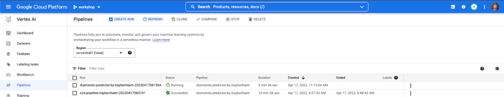
Head over to Vertex in your GCP console and click pipeline, you should see your pipeline:
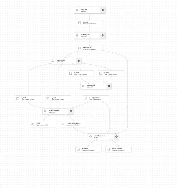
As we said, each of the steps here will have a VM allocated for the runtime, in addition, we can see the outputs and inputs of each step. (I encourage you to explore this to find some easter eggs 🙂 )
Google lets us use many common libraries (tensorflow, sklearn, XGDBoost) out of the box. However, we need to modify it a bit. In this stage, we’ll write a small flask app that will wrap our predictor and log every prediction to our monitoring system.
import logging
import os
from flask import Flask, jsonify, request
from predictor.predictor import DiamondPricePredictor
app = Flask("DiamondPricePredictor")
gunicorn_logger = logging.getLogger("gunicorn.error")
app.logger.handlers = gunicorn_logger.handlers
app.logger.setLevel(gunicorn_logger.level)
predictor = DiamondPricePredictor(os.environ["MODEL_PATH"])
@app.route("/diamonds/v1/predict", methods=["POST"])
def predict():
   """
   Handle the Endpoint predict request.
   """
   predictions = predictor.predict(request.json["instances"])
   return jsonify(
       {
           "predictions": predictions["predicted_prices"],
           "transaction_id": predictions["transaction_id"],
       }
   )
@app.route("/diamonds/v1", methods=["GET"])
def healthcheck():
   """
   Vertex AI intermittently performs health checks on your
   HTTP server while it is running to ensure that it is
   ready to handle prediction requests.
   """
Only 2 endpoints are needed, predict and health check.
The payload for prediction is in the form:
"instances": [
           {
               "carat" : 1.42, "clarity" : "VVS1", "color" : "F", "cut" : "Ideal", "depth" : 60.8, "record_id" : 27671, "table" : 56, "x" : 7.25, "y" : 7.32, "z" : 4.43
           },
           {
               "carat" : 2.03, "clarity" : "VS2", "color" : "G", "cut" : "Premium", "depth" : 59.6, "record_id" : 27670, "table" : 60, "x" : 8.27, "y" : 8.21, "z" : 4.91
           }
           ]
       }
Our predictor script:
import os
from tempfile import TemporaryFile
import joblib
import pandas as pd
from google.cloud import storage
from superwise import Superwise
CLIENT_ID = os.getenv("SUPERWISE_CLIENT_ID")
SECRET = os.getenv("SUPERWISE_SECRET")
SUPERWISE_MODEL_ID = os.getenv("SUPERWISE_MODEL_ID")
SUPERWISE_VERSION_ID = os.getenv("SUPERWISE_VERSION_ID")
class DiamondPricePredictor(object):
   def __init__(self, model_gcs_path):
       self._model = self._set_model(model_gcs_path)
       self._sw = Superwise(
           client_id=os.getenv("SUPERWISE_CLIENT_ID"),
           secret=os.getenv("SUPERWISE_SECRET")
       )
   def _send_monitor_data(self, predictions):
       """
       send predictions and input data to Superwise
       :param pd.Serie prediction
       :return str transaction_id
       """
       transaction_id = self._sw.transaction.log_records(
           model_id=int(os.getenv("SUPERWISE_MODEL_ID")),
           version_id=int(os.getenv("SUPERWISE_VERSION_ID")),
           records=predictions
       )
       return transaction_id
   def predict(self, instances):
       """
       apply predictions on instances and log predictions to Superwise
       :param list instances: [{record1}, {record2} ... {record-N}]
       :return dict api_output: {[predicted_prices: prediction, transaction_id: str]}
       """
       input_df = pd.DataFrame(instances)
       # Add timestamp to prediction
       input_df["predictions"] = self._model.predict(input_df)
       # Send data to Superwise
       transaction_id = self._send_monitor_data(input_df)
       api_output = {
           "transaction_id": transaction_id,
           "predicted_prices": input_df["predictions"].values.tolist(),
       }
       return api_output
   def _set_model(self, model_gcs_path):
       """
       download file from gcs to temp file and deserialize it to sklearn object
       :param str model_gcs_path: Path to gcs file
       :return sklearn.Pipeline model: Deserialized pipeline ready for production
       """
       storage_client = storage.Client()
       bucket_name = os.environ["BUCKET_NAME"]
       print(f"Loading from bucket {bucket_name} model {model_gcs_path}")
       bucket = storage_client.get_bucket(bucket_name)
       # select bucket file
       blob = bucket.blob(model_gcs_path)
       with TemporaryFile() as temp_file:
           # download blob into temp file
           blob.download_to_file(temp_file)
           temp_file.seek(0)
           # load into joblib
           model = joblib.load(temp_file)
       print(f"Finished loading model from GCS")
       return model
Our predictor implements 3 functions:
FROM python:3.7
WORKDIR /app
COPY requirements.txt ./
RUN pip install -r requirements.txt
COPY . ./
ARG MODEL_PATH
ARG SUPERWISE_CLIENT_ID
ARG SUPERWISE_SECRET
ARG SUPERWISE_MODEL_ID
ARG SUPERWISE_VERSION_ID
ARG BUCKET_NAME
ENV SUPERWISE_CLIENT_ID=${SUPERWISE_CLIENT_ID}
ENV SUPERWISE_SECRET=${SUPERWISE_SECRET}
ENV BUCKET_NAME=${BUCKET_NAME}
ENV MODEL_PATH=${MODEL_PATH}
ENV SUPERWISE_MODEL_ID=${SUPERWISE_MODEL_ID}
ENV SUPERWISE_VERSION_ID=${SUPERWISE_VERSION_ID}
ENV FLASK_APP /app/server.py
ENV GOOGLE_APPLICATION_CREDENTIALS /app/resources/creds.json
ENTRYPOINT ["gunicorn", "--bind", "0.0.0.0:5050", "predictor.server:app", "--timeout", "1000", "-w", "4"]
EXPOSE 5050
Now we need to push this to a new artifactory registry in GCP.
Go to GCP console -> artifact registry -> create repository
name: diamonds-predictor-repo
format: docker
Then run this in terminal
REPOSITORY='diamonds-predictor-repo'
PROJECT_ID='your GCP project ID'
REGION='<GCP Region (e.g. us-central 1)>'
IMAGE='diamonds_predictor'
docker build --tag=${REGION}-docker.pkg.dev/${PROJECT_ID}/${REPOSITORY}/${IMAGE} .
docker push ${REGION}-docker.pkg.dev/${PROJECT_ID}/${REPOSITORY}/${IMAGE}
Register your model to Superwise:
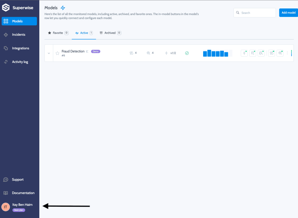
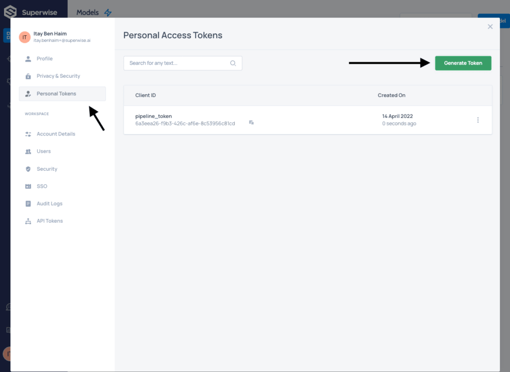
In order to monitor your model in production, you’ll first need to register it to Superwise’s platform. For this step, we will need to log into Superwise and generate a CLIENT_ID and a SECRET. Click on your user name on the bottom left.
Then select personal tokens and generate a token, copy the CLIENT ID and SECRET, and save it somewhere safe.
The following snippet is a new component designed to register your model to Superwise, create a version for it (similar to a tag) and have Superwise stand ready to monitor it.
SUPERWISE_CLIENT_ID="<YOUR SUPERWISE ACCOUNT CLIENT ID>" # @param project number
SUPERWISE_SECRET="<YOUR SUPERWISE ACCOUNT SECRET>"# @param project number
SUPERWISE_MODEL_NAME = "Regression - Diamonds Price Predictor"
@component(packages_to_install=["superwise", "pandas"])
def register_model_to_superwise(
    model_name: str,
    superwise_client_id: str,
    superwise_secret: str,
    baseline: Input[Dataset],
    timestamp: str,
) -> NamedTuple("output", [("superwise_model_id", int), ("superwise_version_id", int)]):
    import pandas as pd

    from datetime import datetime
    from superwise import Superwise
    from superwise.models.model import Model
    from superwise.models.version import Version
    from superwise.resources.superwise_enums import DataEntityRole
    from superwise.controller.infer import infer_dtype
    sw = Superwise(
        client_id=superwise_client_id,
        secret=superwise_secret,
    )
    first_version = False
    # Check if model exists
    models = sw.model.get_by_name(model_name)
    if len(models) == 0:
        print(f"Registering new model {model_name} to Superwise")
        diamond_model = Model(name=model_name, description="Predicting Diamond Prices")
        new_model = sw.model.create(diamond_model)
        model_id = new_model.id
        first_version = True
    else:
        print(f"Model {model_name} already exists in Superwise")
        model_id = models[0].id
    baseline_data = pd.read_csv(baseline.path).assign(
        ts=pd.Timestamp.now() - pd.Timedelta(30, "d")
    )
    # infer baseline data types and calculate metrics & distribution for features
    entities_dtypes = infer_dtype(df=baseline_data)
    entities_collection = sw.data_entity.summarise(
        data=baseline_data,
        entities_dtypes=entities_dtypes,
        specific_roles={
            "record_id": DataEntityRole.ID,
            "ts": DataEntityRole.TIMESTAMP,
            "predictions": DataEntityRole.PREDICTION_VALUE,
            "price": DataEntityRole.LABEL,
        },
    )
    if not first_version:
        model_versions = sw.version.get({"model_id": model_id})
        print(
            f"Model already has the following versions: {[v.name for v in model_versions]}"
        )
    new_version_name = f"v_{timestamp}"
    # create new version for model in Superwise
    diamond_version = Version(
        model_id=model_id,
        name=new_version_name,
        data_entities=entities_collection,
    )
    new_version = sw.version.create(diamond_version)
    # activate the new version for monitoring
    sw.version.activate(new_version.id)
    return (model_id, new_version.id)
Our inputs are the model_id, client and secret, the baseline data that we performed the training on, and a timestamp to create a unique version name. The code above uses the Superwise public SDK to perform actions on the platform.
Our final step will be to create the endpoint and deploy our custom image to it.
@component(
    packages_to_install=[
        "google-cloud-aiplatform==1.7.0",
        "google-cloud-pipeline-components",
    ]
)
def deploy_model_to_endpoint(
    project: str,
    location: str,
    bucket_name: str,
    timestamp: str,
    superwise_client_id: str,
    superwise_secret: str,
    superwise_model_id: int,
    superwise_version_id: int,
    serving_container_image_uri: str,
    model: Input[Model],
    vertex_model: Output[Model],
):
    import os
    from google.cloud import aiplatform, storage
    aiplatform.init(project=project, location=location)
    DISPLAY_NAME = "Diamonds-Price-Predictor"
    def create_endpoint():
        endpoints = aiplatform.Endpoint.list(
            filter='display_name="{}"'.format(DISPLAY_NAME),
            order_by="create_time desc",
            project=project,
            location=location,
        )
        if len(endpoints) > 0:
            endpoint = endpoints[0]  # most recently created
        else:
            endpoint = aiplatform.Endpoint.create(
                display_name=DISPLAY_NAME, project=project, location=location
            )
        return endpoint
    def upload_model_to_gcs(artifact_filename, local_path):
        model_directory = f"{bucket_name}/models/"
        storage_path = os.path.join(model_directory, artifact_filename)
        blob = storage.blob.Blob.from_string(storage_path, client=storage.Client())
        blob.upload_from_filename(local_path)
        return f"models/{artifact_filename}"
    endpoint = create_endpoint()
    model_gcs_path = upload_model_to_gcs(f"model_{timestamp}.joblib", model.path)
    model_upload = aiplatform.Model.upload(
        display_name=DISPLAY_NAME,
        serving_container_image_uri=serving_container_image_uri,
        serving_container_ports=[5050],
        serving_container_health_route=f"/diamonds/v1",
        serving_container_predict_route=f"/diamonds/v1/predict",
        serving_container_environment_variables={
            "MODEL_PATH": model_gcs_path,
            "BUCKET_NAME": bucket_name.strip("gs://"),
            "SUPERWISE_CLIENT_ID": superwise_client_id,
            "SUPERWISE_SECRET": superwise_secret,
            "SUPERWISE_MODEL_ID": superwise_model_id,
            "SUPERWISE_VERSION_ID": superwise_version_id,
        },
    )
    print("uploaded version")
    model_deploy = model_upload.deploy(
        machine_type="n1-standard-4",
        endpoint=endpoint,
        traffic_split={"0": 100},
        deployed_model_display_name=DISPLAY_NAME,
    )
    vertex_model.uri = model_deploy.resource_name
During this step’s execution, we will write the serialized model object using joblib into a predefined folder in the bucket (not the pipeline’s root), so the predictor will be able to run_set_model function and load it from there. In addition, we will deploy the image using all the environment variables needed for it to work.
Lastly, in this code snippet, we can see that the deploy function gets a machine-type (we chose the basic one), and a traffic split, which is useful for A/B testing or gradual deployments.
At last, we’re here! Let’s create a new pipeline and run it!
@pipeline(
    name=PIPELINE_NAME,
    description="An ml pipeline",
    pipeline_root=PIPELINE_ROOT,
)
def ml_pipeline():
    raw_data = load_data()
    validated_data = validate_data(raw_data.outputs["dataset"])
    prepared_data = prepare_data(validated_data.outputs["validated_df"])
    trained_model_task = train_model(
        prepared_data.outputs["X_train"], prepared_data.outputs["y_train"]
    )
    evaluated_model = evaluate_model(
        trained_model_task.outputs["model_artifact"],
        prepared_data.outputs["X_test"],
        prepared_data.outputs["y_test"],
    )
    validated_model = validate_model(
        new_model_metrics=evaluated_model.outputs["model_performance"],
        new_model=trained_model_task.outputs["model_artifact"],
        dataset=validated_data.outputs["validated_df"],
    )
    ### NEWLY ADD SECTION ###
    with dsl.Condition(
        validated_model.outputs["deploy"] == "true", name="deploy_decision"
    ):
        superwise_metadata = register_model_to_superwise(
            SUPERWISE_MODEL_NAME,
            SUPERWISE_CLIENT_ID,
            SUPERWISE_SECRET,
            validated_model.outputs["baseline"],
            TIMESTAMP,
        )
        vertex_model = deploy_model_to_endpoint(
            PROJECT_ID,
            REGION,
            BUCKET_NAME,
            TIMESTAMP,
            SUPERWISE_CLIENT_ID,
            SUPERWISE_SECRET,
            superwise_metadata.outputs["superwise_model_id"],
            Superwise_metadata.outputs["superwise_version_id"],
            f"{REGION}-docker.pkg.dev/{PROJECT_ID}/diamonds-predictor-repo/diamonds_predictor:latest",
            trained_model_task.outputs["model_artifact"],
        )
Exactly like the pipeline we already executed, with 3 new lines
dsl.condition helps us set conditions during execution. In our case, if the evaluation step were producing a False value, we would not continue to deployment.
Superwise_metadata – Gets the outputs of the register_model_to_superwise step
Vertex_model – Get a single output, the vertex_model uri. We will use this to send prediction requests.
Let’s run it:
def upload_blob(bucket_name, source_file_name, destination_blob_name):
    """Uploads a file to the bucket."""
    storage_client = storage.Client(project=PROJECT_ID)
    bucket = storage_client.get_bucket(bucket_name)
    blob = bucket.blob(destination_blob_name)
    blob.upload_from_filename(source_file_name)
    print("File {} uploaded to {}.".format(source_file_name, destination_blob_name))
TIMESTAMP = datetime.now().strftime("%Y%m%d%H%M%S")
ml_pipeline_file = "ml_pipeline.json"
compiler.Compiler().compile(
    pipeline_func=ml_pipeline, package_path=ml_pipeline_file
)
job = aiplatform.PipelineJob(
    display_name="diamonds-predictor-pipeline",
    template_path=ml_pipeline_file,
    job_id="e2e-pipeline-{}-{}".format(USERNAME, TIMESTAMP),
    enable_caching=True,
)
upload_blob(
    bucket_name=BUCKET_NAME.strip("gs://"),
    source_file_name=ml_pipeline_file,
    destination_blob_name=ml_pipeline_file,
)
job.submit()
In this execution snippet, we added a small function to upload the generated JSON file to GCS as well, so other users can use it or in case we want to perform a rollback and load an older model.
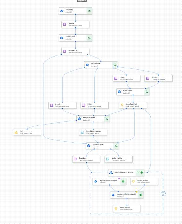
This will run for a few minutes. Vertex will use a caching mechanism to skip the first pipeline we ran and execute only the 2 new steps. Here’s how the graph should look once it’s done:
In order to simulate a web server listening to events and triggering a new pipeline in case of an incident. I will be using Google’s cloud function in order to trigger the webhook. This webhook will trigger a new pipeline, only this time, our extract_data component will read the entire Diamonds dataset, so our model will encounter >10000 priced diamonds.
To do so, I have placed a file called full_data_ml_pipeline.json (which is the output of our pipeline.py script) without the df = df[df[‘price’] < 10000] line, in “gs://pipeline_blog_bucket/itaybenhaim_pipeline_root/full_data_ml_pipeline.json”
Head over to GCP cloud functions, enable the requested APIs, and create a new HTTP function with Python code:
from google.cloud import aiplatform
PROJECT_ID = 'your-project-id'                     # <---CHANGE THIS
REGION = 'your-region'                             # <---CHANGE THIS
PIPELINE_ROOT = 'your-cloud-storage-pipeline-root' # <---CHANGE THIS
def trigger_pipeline_run():
    """Triggers a pipeline run"""
    pipeline_spec_uri = "gs://pipeline_blog_bucket/itaybenhaim_pipeline_root/full_data_ml_pipeline.json"
    # Create a PipelineJob using the compiled pipeline from pipeline_spec_uri
    aiplatform.init(
        project=PROJECT_ID,
        location=REGION,
    )
    job = aiplatform.PipelineJob(
        display_name='incident-triggered-ml-pipeline',
        template_path=pipeline_spec_uri,
        pipeline_root=PIPELINE_ROOT,
        enable_caching=False
    )
    # Submit the PipelineJob
    job.submit()
We will use the generated URL of this webhook in Superwise’s integrations page:
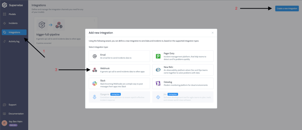
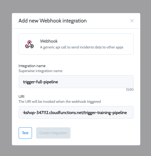
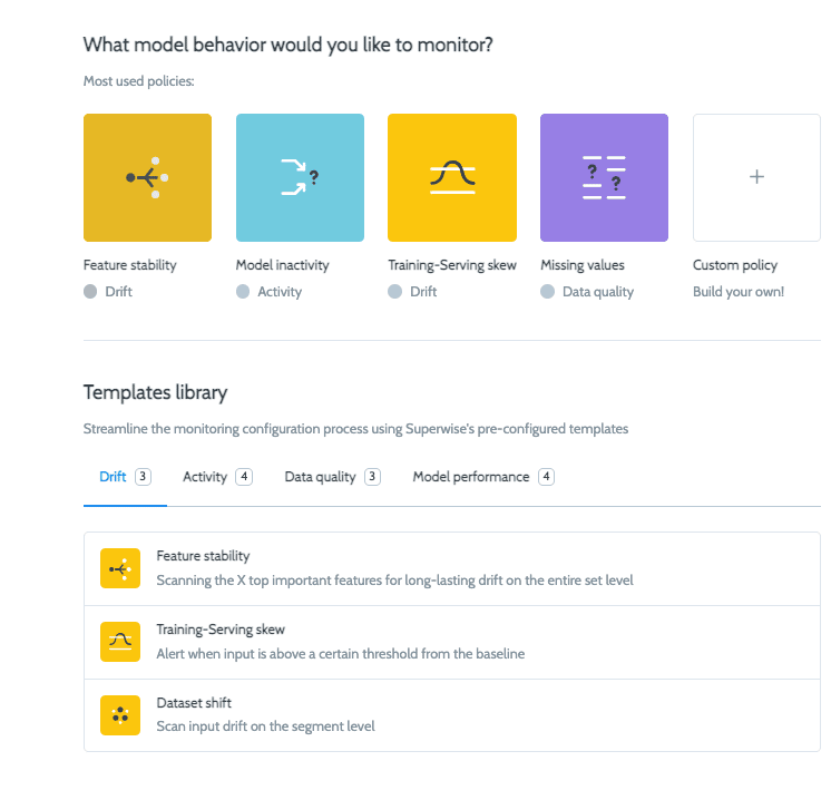
Now let’s create a policy in Superwise so that upon violation detection will trigger a webhook to retrain our pipeline. On the main models page, click on add monitoring policy.
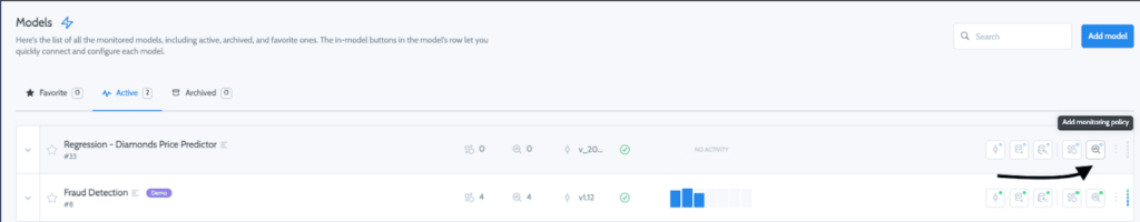
Then follow the wizard to configure a policy and integrate it into the trigger-full-pipeline webhook (I chose feature stability and had Superwise automatically configure the thresholds and features to monitor).
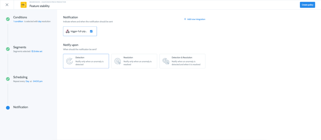
Great! We are all set, and our Vertex endpoint is being monitored!
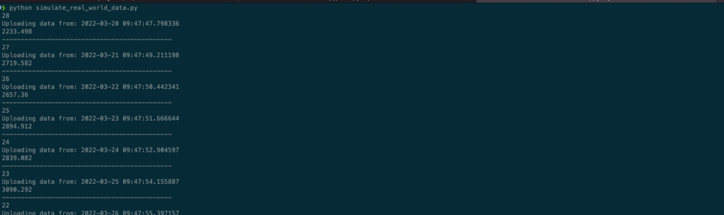
Now let’s simulate real-world behavior of a production environment.
Let’s say that in the first 18 days of use, the new observations were in the range of <10000 priced diamonds, and the model performed well, but lo and behold, a new diamond mine has been revealed, causing diamonds to be bigger and raise their prices!!
(In a new script)
import requests
import json
import pandas as pd
import google.auth
import google.auth.transport.requests
ENDPOINT_ID = "<GET THE ENDPOINT_ID FROM THE PIPELINE'S OUTPUT>" # @param
url = f"https://{REGION}-aiplatform.googleapis.com/v1/projects/{PROJECT_NUMBER}/locations/{REGION}/endpoints/{ENDPOINT_ID}:predict"

credentials, project_id = google.auth.default(
    scopes=[
        "https://www.googleapis.com/auth/cloud-platform",
        "https://www.googleapis.com/auth/cloud-platform.read-only",
    ]
)
instances = {"instances": []}
df = pd.read_csv("https://www.openml.org/data/get_csv/21792853/dataset")
expensive_df = df[df["price"] > 10000].sort_values("price", ascending=False)
df = df[df["price"] < 10000]
count = 28
chunk_size = 500
reset_index = True
min_chunk, max_chunk = 0, chunk_size
while count:
    print(count)
    print(f"Uploading data from: {str(pd.Timestamp.now() - pd.Timedelta(count, 'd'))}")
    if count < 10:
        if reset_index:
          min_chunk, max_chunk = 0, 500
          reset_index = False
        print(expensive_df.iloc[min_chunk:max_chunk]['price'].mean())
        for row_tuple in expensive_df.iloc[min_chunk:max_chunk].iterrows():
            row_dict = row_tuple[1].drop("price").to_dict()
            row_dict["record_id"] = row_tuple[1].name
            row_dict["ts"] = str(pd.Timestamp.now() - pd.Timedelta(count, 'd'))
            instances["instances"].append(row_dict)
    else:
        print(df.iloc[min_chunk:max_chunk]['price'].mean())
        for row_tuple in df.iloc[min_chunk:max_chunk].iterrows():
            row_dict = row_tuple[1].drop("price").to_dict()
            row_dict["record_id"] = row_tuple[1].name
            row_dict["ts"] = str(pd.Timestamp.now() - pd.Timedelta(count, 'd'))
            instances["instances"].append(row_dict)
    request = google.auth.transport.requests.Request()
    credentials.refresh(request)
    token = credentials.token
    headers = {"Authorization": "Bearer " + token}
    response = requests.post(url, json=instances, headers=headers)
    #print(response.text) ## If needed 🙂
    print("---" * 15)
    instances["instances"] = []
    count -= 1
    min_chunk += chunk_size
    max_chunk += chunk_size
Running this will generate the situation above and have Superwise trigger a webhook to retrain on the whole dataset!
Output:
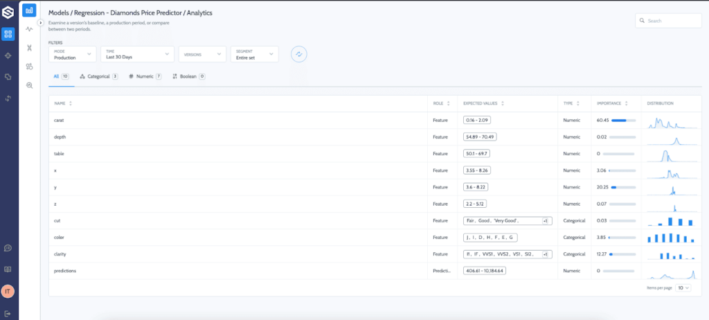
Before we look into the incidents and the automation, we can see Superwise has calculated the production data distributions for us, and we can already see a distribution shift in multiple features.
Now the incident will get caught when the policy daemon will run (according to the schedule defined in the policy) and show up on the incidents screen.
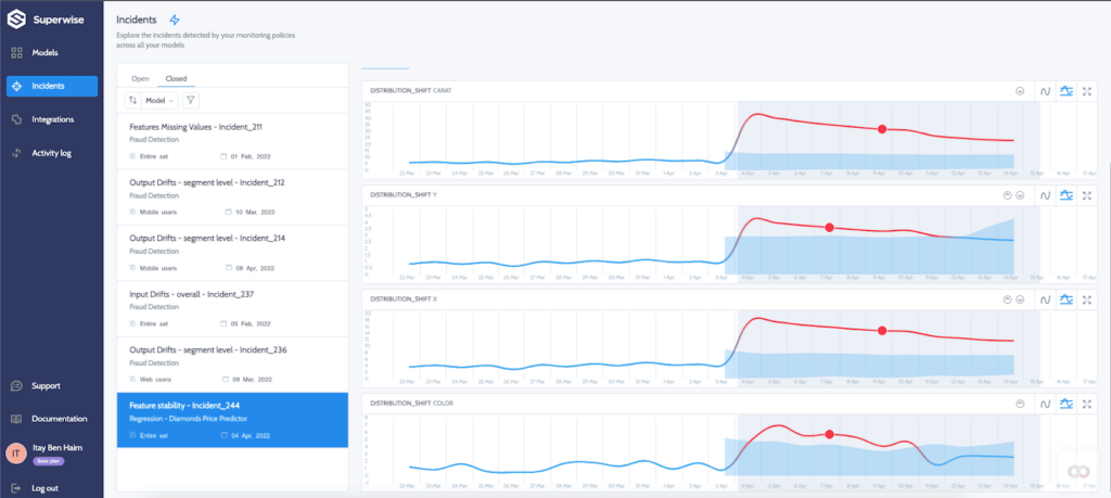
Superb!! We simulated the distribution shift, and Superwise automatically triggered our cloud function to rerun the training pipeline:
In this super yet awesomely long post, we introduced two new paradigms:
The stack and the technical implementation can be adapted and assembled from many different tools. There are a lot of great off-the-shelf and open-source tools out there, so it’s entirely up to you to put together the toolbox that best fits your needs! Using the big vendors’ ML platforms is a quick and easy way to get started but is less flexible and will not always work for some use cases.
And one final thing to think about before we sign off. Retraining is not always the solution. Sometimes model recalibration, fixing the data source stream, splitting to sub-populations, and adjusting thresholds are needed. So you need to ensure that the monitoring you set up is capable of detecting issues, identifying root-cause, and identifying the right resolution needed.
For any questions, discussions, or ideas – talk to us!
We all know that our model’s best day in production will be its first day in production. It’s simply a fact of life that, over time, model performance degrades. ML attempts to predict real-world behavior based on observed patterns it has trained on and learned. But the real world is dynamic and always in motion; sooner or later, depending on your use case and data velocity, your model will decay and begin to exhibit concept drift, data drift, or even both.

When models misbehave, we often turn to retraining to attempt to fix the problem. As a rule of thumb, data science teams will often take the most recent data from production, say 2 or 3 months’ worth of data, and retrain their model on it with the assumption that “refreshing” the model’s training observations will enable it to predict future results better. But is the most recent data the best data to resolve a model’s performance issues and get it back on track? Think about it this way, if an end-to-end software test failed would you accept it as fixed just by rerunning the test? Most likely not. You’d troubleshoot the issue to pinpoint the root cause and apply an exact fix to resolve the issue. ML teams do precisely this with model monitoring to pinpoint anomalies and uncover their root cause to resolve issues quickly before they impact business outcomes. But when the resolution requires retraining, “fresh is best” is not exactly a data-driven approach.
This article will demonstrate how data science and ML engineering teams can leverage ML monitoring to find the best data and retraining strategy mix to resolve machine learning performance issues. This data-driven, production-first approach enables more thoughtful retraining selections and shorter and leaner retraining cycles and can be integrated into MLOps CI/CD pipelines for continuous model retraining upon anomaly detection.
The insights explained below are based on anomalies detected in the Superwise model observability platform and analyzed in a corresponding jupyter notebook that extracts retraining insights. All the assets are open for use under the Superwise community edition, and you can use it to run the notebook on your own data.
* It’s important to note that the value of this approach lies in identifying how to best retrain once you have eliminated other possible issues in your root cause investigation.
The question? What data should I use for the next retraining?
Models are subject to temporality and seasonality. Selecting a dataset impacted by a temporal anomaly or flux can result in model skew. An important insight from production data is data DNA or the similarity of days distribution. Understanding how data is changing between dates (drift score between dates) enables date-based grouping based on similarities and differences. With this information, you can create a combination of data-retraining groups that reflect or exclude the temporal behavior of your production data.
Here we can see a heatmap plot matrix of dates X dates, and each cell represents the change between 2 dates. Cells colored in bold are very different from each other, while cells that are colored lightly represent dates that are very similar to each other.

As you can see in this example, the data is divided into 3 main groups, orange, red, and green, representing the 3 optional datasets to use in the next retraining.
Depending on your domain insights, the include/exclude decisions may differ. If the marketing campaign was successful and the insights will be rolled-out to all marketing campaigns, you may decide to retrain green and red. If the campaign was a one-time event or a failed experiment, orange and red would be a better retraining data group selection.

The question? Which populations are impacted?
A model’s purpose is to abstract predictions across your population, but with that said, you will always need to monitor your model’s behavior on the segment level to detect if a specific segment is drifting. When segment drift is detected, we can consider the following resolutions or even a combination of them, together with retraining.
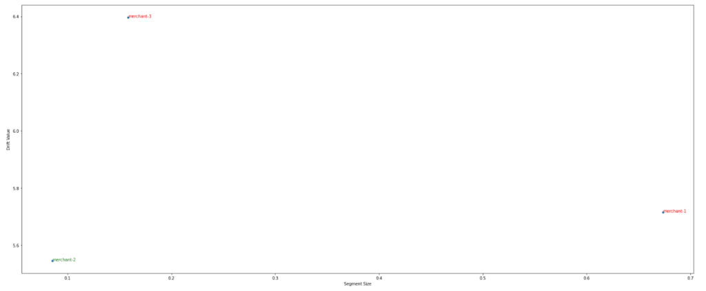
Here we can see the segment drift value where each bar shows the drift score of each segment. Before taking action, it is important to understand the relationship of the segment size to the segment drift to determine the extent of the segment’s effect on the model.
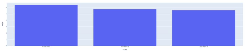
Moreover, this lets us see the relation of segment size to the segment drift value and determine if we need to create a specific model for this segment or not.
The question? Which days should be excluded from retraining on principle?
Some data should be excluded from retraining on principle, namely days when we experienced data integrity issues due to some pipeline or upstream source issue. If this data is taken into consideration during retraining, it can cause our model to misinterpret the ‘normal’ distribution, which can result in a further decline in model performance.
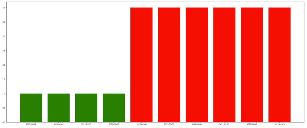
Here we can see a bar graph of the days with data integrity incidents. This lets us quickly identify ‘bad’ data that we should exclude from the next retraining.
Retraining isn’t free. It takes up resources both in terms of training runs and your team’s focus and efforts. So anything that we can do to improve the probability of finishing a retraining cycle with higher-performing results is crucial. That is the value of data-driven retraining with production insights. Smarter and leaner retraining that leverages model observability to take you from detection quickly and effectively.
Head over to the Superwise platform and get started with easy, customizable, scalable, and secure model observability for free with our community edition.
Request a demo and our team will show what Superwise can do for your ML and business.