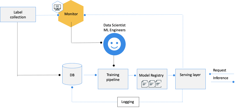
Framework for a successful continuous training strategy

ML models are built on the assumption that the data used in production will be similar to the data observed in the past, the one that we trained our models on. While this may be true for some specific use cases, most models work in dynamic data environments where data is constantly changing and where “concept drifts” are likely to happen and adversely impact the models’ accuracy and reliability.
To deal with this, ML models need to be retrained regularly. Or as stated in Google’s “MLOps: Continuous delivery and automation pipelines in machine learning“: “To address these challenges and to maintain your model’s accuracy in production, you need to do the following: Actively monitor the quality of your model in production […] and frequently retrain your production models.” This concept is called ‘Continuous Training’ (CT) and is part of the MLOps practice. Continuous training seeks to automatically and continuously retrain the model to adapt to changes that might occur in the data.
There are different approaches/methodologies to perform continuous retraining, each with its own pros, cons, and cost. Yet, similar to the shoemaker who walks barefoot, we – data scientists – seem to overdo retraining, sometimes manually, and often use it as a “default” solution without enough production-driven insights.
Each ML use case has its own dynamic data environment that can cause concept drifts: from real-time trading to fraud detection, with the adversary changing the data distribution or recommendation engines with a wealth of new movies and new trends. Yet, regardless of the use case, three main questions need to be addressed when designing a continuous training strategy:
1 – When should the model be retrained? As the goal is to keep running models that are highly relevant and that perform optimally at any point in time, how often should the model be retrained
2 – What data should be used? The common assumption for the selection of the adequate dataset is that the relevance of the data is correlated to how recent it is, which triggers a set of questions: should we use new data or add to older data sets? What is a good balance between old and new data? How recent is considered new data, or when is the cut between old and new data?
3 – What should be retrained? Can we replace data and retrain the same model with the same hyperparameters? Or should we take a more intrusive approach and run a full pipeline that simulates our research process?
Each of the three questions above can be answered separately, and can help determine the optimal strategy for each case. Yet, and while answering these questions, there is a list of considerations that need to be taken into account, and which we have investigated herein. For each question, we describe different approaches, corresponding to different levels of automation and maturity of the ML process.
When to retrain?
The three most common strategies are periodic retraining, performance-based, or based on data changes.
Periodic retraining
A periodic retraining schedule is the most naive and straightforward approach. Usually, it is time-based: the model is retrained every 3 months – but can also be volume-based – i.e., for every 100K new labels.
The advantages of periodic retraining are just as straightforward: this is a very intuitive and manageable approach as it is easy to know when the next retraining iteration will happen, and it is easy to implement.
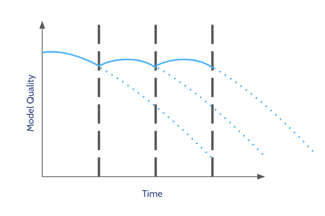
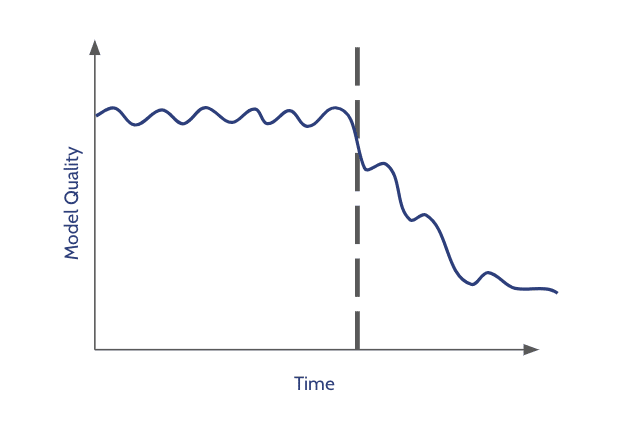
This method, though, often reveals itself to be ill-fitted or inefficient. How often do you retrain the model? Every day? Every week? Every three months? Once a year? While one may want to frequently retrain to keep models up-to-date, retraining the model too often when there is no actual reason, i.e., no concept drift, is costly. Besides, even when retraining is automated, it requires important resources – both computational and from your data science teams who need to oversee the retraining process and the new model behavior in production after deployment. Yet, retraining with large intervals may miss the point of continuous retraining and fail to adapt to changes in the data without mentioning the risks of retraining on noisy data.
At the end of the day, a periodic retraining schedule makes sense if the frequency is aligned with the dynamism of your domain. Otherwise, the selection of a random time/milestone may expose you to risks and leave you with models that have less relevance than their previous version.
Performance-based trigger
It’s almost a common-sense claim based on the good old engineering adage: “if it ain’t broken, don’t fix it.” The second most common approach to determine when to retrain is to leverage performance-based triggers and retrain the model once you detect performance degradation.
This approach, more empirical than the first one, assumes that you have a continuous view of the performance of your models in production.
The main limitation when relaying on performance only is the time it takes for you to obtain your ground truth – if you obtain it at all. In user conversion prediction cases, it can take 30 or 60 days until you will get a ground truth, or even 6 months or more in cases such as transaction fraud detection or LTV. If you need to wait so long to have full feedback, that means you’ll retrain the model too late after the business has already been impacted.
Another non-trivial question that needs to be answered is: what is considered ‘performance degradation’? you may be dependent on the sensitivity of your thresholds and the accuracy of the calibration, which could lead you to retrain too frequently or not frequently enough.
Overall, using performance based triggers is good for use-cases where there is fast feedback and high volume of data, like real time bidding, where you are able to measure the model’s performance as close as possible to the time of predictions, in short time intervals and with high confidence (high volume).
Driven by data changes
This approach is the most dynamic and naturally triggers retraining from the dynamism of the domain. By measuring changes in the input data, i.e., changes in the distribution of features that are used by the model, you can detect data drifts that indicate your model may be outdated and needs to be retained on fresh data.
It is an alternative to the performance-based approach for cases where you don’t have fast feedback or cannot assess the performance of the model in production in real-time. Besides, it’s also a good practice to combine and use this approach even when there is fast feedback, as it may indicate suboptimal performance, even without degradation. Understanding data changes to start a retraining process is very valuable, especially in dynamic environments.
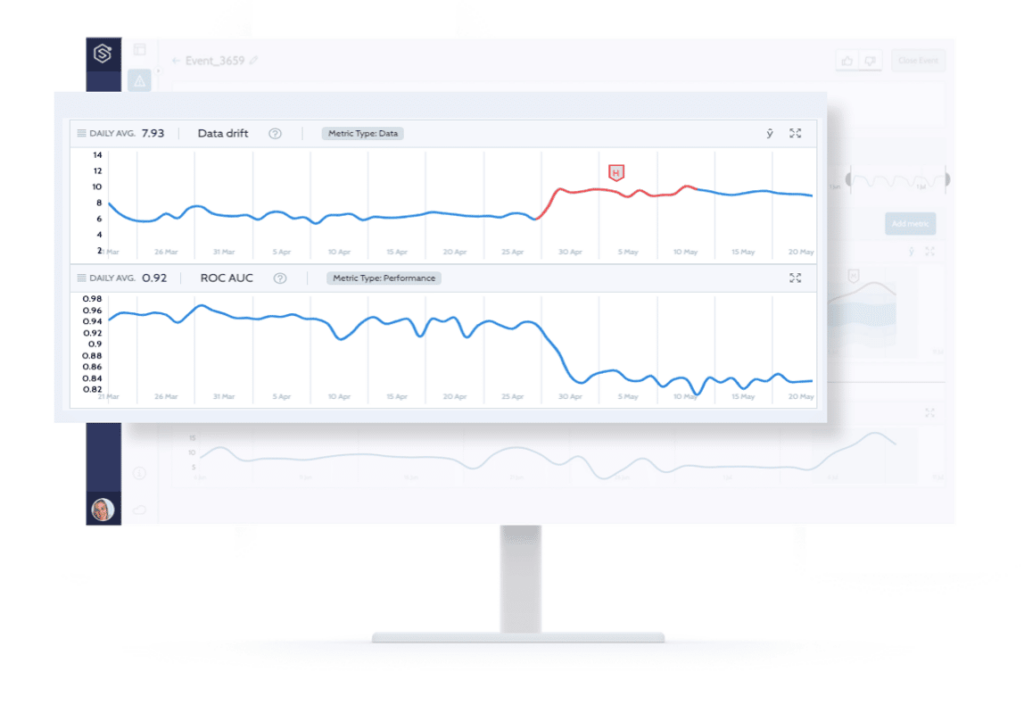
The graph above, generated by the monitoring service, shows a data drift metric (upper graph) and a performance KPI (lower graph) on a marketing use case. The data drift graph is a timeline where the Y-axis shows the level of drift for each day (i.e., the data on this day) relative to the training set. In this marketing use-case example, new campaigns are introduced very frequently, and the business expands to new countries. Clearly, the data streaming in production is drifting and becoming less similar to the data on which the model was trained. By having a more thorough view of the model in production, a retraining iteration could have been triggered well before a performance degradation would have been observed by the business.
So when to retrain? This depends on key factors such as: the availability of your feedback, the volume of your data, and your visibility on the performance of your models. Overall, there is no one size fits all to the question of selecting the right time to retrain. Rather, and depending on your resources, the goal should be to be as production driven as possible.
What data should be used?
While we have seen that timing is everything (i.e., when do I retrain my models?), now let’s look at the nerve of all MLOps: the data. When retraining, how do I select the right data to be used?
Fix window size
The most naive approach is to use a fixed window size as a training set. For example, use data from the last X months. Clearly, the advantage of the method is in its simplicity, as it is very straightforward.
The disadvantages derive from the challenge of selecting the right window: if it is too wide, it may miss new trends, and if it is too narrow, it will be overfitted and noisy. The choice of the window size should also take into account the frequency of retraining: it makes no sense to retrain every 3 months if you only use the last month of data as a training set.
Besides, the data selected can be very different from the data that is being streamed in production, as it may happen straight after a change point (in case of fast/sudden change), or it may contain irregular events (e.g., holidays or special days like election day), data issues and more.
Overall, the fix window approach, like any other “static” method, is a simple heuristic which may work well in some cases, but will fail to capture the hyper dynamism of your environment in cases where the change rate is versatile and irregular events are common like holidays or technical issues.
Dynamic window size
The dynamic window size approach tries to solve some of the limitations of the predefined window size by determining how much historical data should be included in a more data-driven way and by treating the window size as another hyperparameter that can be optimized as part of the retraining.
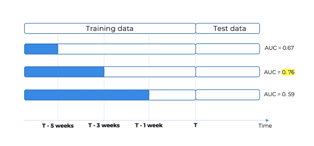
This approach is most suitable for cases in which there is fast feedback (i.e., Real-Time Bidding or food delivery ETA). The most relevant data can be used as a test set, and the window size can be optimized on it, just like another hyperparameter of the model. In the case illustrated below, the highest performance is achieved by taking the last 3 weeks, which is what should be selected for this iteration. For future ones, a different window may be selected according to the comparison with the test set.
The advantage of the dynamic window size approach is that it is more data-driven, based on the model performance, which is really the bottom line, and hence it is more robust for highly temporal environments.
The disadvantage is that it requires a more complex training pipeline (see next question ‘What to train’) to test the different window sizes and select the optimal one, and it is much more computing-intensive. Additionally, like the fixed window size, it assumes that the most recent data is the most relevant, which is not always true.
Dynamic data selection
The third approach of selecting the data to train the models seeks to achieve the basic objective of any retraining strategy, which is the basic assumption of any ML model: using training data that is similar to the production data. Or in other words, models should be retrained on data that is as similar as possible to the data used in real-life to issue predictions. This approach is complex and requires high visibility of the production data.
To do so, you need to perform a thorough analysis of the evolution of the data in production to understand if and how it changes over time. One way to do this is to calculate the drift in input data between each pair of days, i.e., how much the data of one day is different from the data of another day, and generate a heat map that reveals the change patterns of the data over time like the one shown below. The heat map below is a visualization of drift evaluation over time where the axes (columns and rows) are dates, and each dot (cell in the matrix) is the level of drift between two days, where the higher the drift, the more red the cell is.
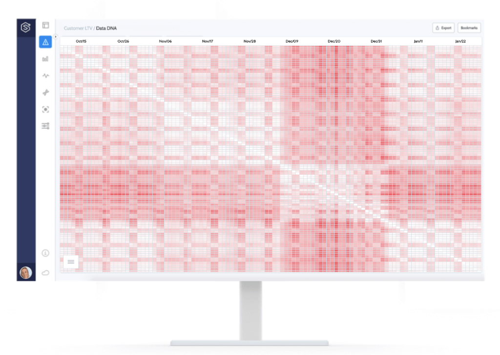
Above, you can see the result of such an analysis generated automatically by Superwise to help spot data that is as similar as possible to the one that is now streaming. There are different types of insights that can transpire easily from this view:
1 – The month of December is very different from the rest of the data (before and after). This insight enables us to avoid treating the whole period as bulk and exclude these days when you want to retrain, as this month’s data doesn’t represent the normal data you observe in production.
2- The seasonality of the data can be visualized – and this can trigger a discussion around the necessity to use different models for weekdays and weekends.
One more thing that is very powerful here: you can actually have a picture that proves that the most recent data isn’t necessarily the most relevant.
In short, selecting the right data to retrain your models requires a thorough view of the behavior of the data in production. While using fixed or dynamic window sizes may help you to “tick the box”, it usually remains a guesstimation that might be more costly than efficient.
What should be retrained?
Now that we have analyzed when to retrain and what data should be used let’s address the third question: what should be retrained? One could select only to retrain (refit) the model instance based on the new data, to include some or all of the data preparation steps, or take a more intrusive approach and run a full pipeline that simulates the research process.
The basic assumption of retraining is that the model that was trained in the research phase will become outdated due to concept drift and hence need to be retrained. However, in most cases, the model instance is just the last phase of a wider pipeline that was built in the research phase and includes data preparation steps. The question is: how severe is the drift and its impact? or in the context of retraining, what parts of the model pipeline should be challenged?
In the research phase, you experiment and evaluate many elements within the model pipeline steps in an effort to optimize your model. These elements can be grouped into two high-level parts, data preparation, and model training. The data preparation part is responsible for preparing the data (duh!) to be consumed by the model and includes methods like feature engineering, scaling, imputation, dimensional reduction, etc., and the model training part is responsible for selecting the optimal model and its hyperparameters. At the end of the process, you get a pipeline of sequential steps that take the data, prepare it to be used by the model and predict the target outcome using the model.
Retraining only the model, i.e., the last step in the pipeline, with new relevant data is the most simple and naive approach and may suffice to avoid performance degradation. However, in some cases, this model-only approach may not be enough, and a more comprehensive approach should be taken regarding the scope of the retraining. Broadening the scope of retraining can be performed in two dimensions:
1 – What to retrain? What parts of the pipeline should be retrained using the new data?
2 – Level of retraining: Are you just refitting the model (or other steps) with the new data? Do you do hyperparameters optimization? or do you challenge the selection of the model itself and test for other model types?
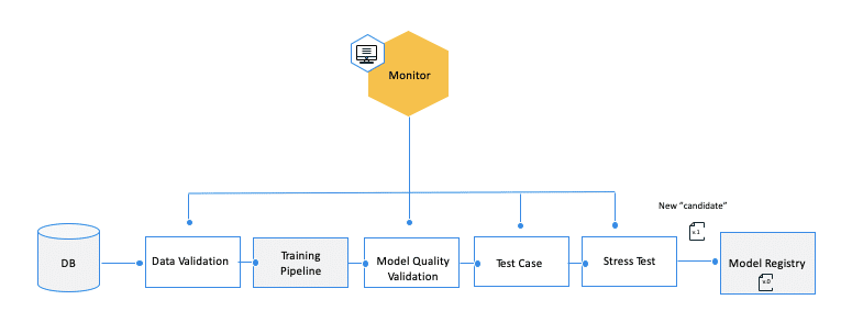
Another way to look at this is that in the retraining process, you basically try to automate and avoid the manual work of model optimization research that would be done by a data scientist if there was no automatic retraining process. Hence you need to decide to what extent you want to try and mimic the manual research process, as illustrated in the chart below.
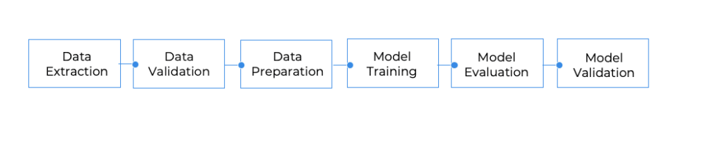
Note that automating the first steps of the flow is more complex, and as more automation is built around these experimentations, the process grows more robust and flexible to adapt to changes, but it also adds complexity as more end cases and checks should be considered
Example & conclusion
Let’s take, for example, a simple model pipeline that is a result of manual research done by our awesome data science team for some classification tasks:
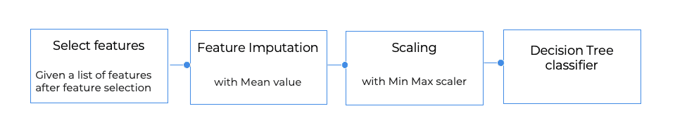
You can take the simple approach and retrain the model itself and let it learn a new tree, or you can include some (or all) data preparation steps (e.g., relearn the mean in the imputer or the min/max values in the scaler). But besides the selection of the steps to be retrained, you need to decide to what level. For example, even if you choose to retrain just the model, it can be performed on multiple levels. You can retrain the model itself and let it learn a new tree, i.e., model fit (new_X, new_y), or you can search and optimize the model hyperparameters (max depth, min leaf size, max-leaf nodes, etc.) or even challenge the selection of the model itself and test for other model types (e.g., logistic regression and. random forest). The data preparation steps can (and should) also be retrained to test for different scalers or different imputation methods or even test for different feature selections.
When choosing to take the more comprehensive approach and perform hyperparameter optimization/model search, you can also use AutoML frameworks that are designed to automate the process of building and optimizing the model pipeline, including data preparation, model search, and hyperparameter optimization. And it doesn’t have to involve complex meta-learning. It can be simple: the user selects a range of models and parameters. A lot of tools are available: AutoKeras, Auto SciKitLearn. Yet, as tempting as AutoML is, it doesn’t exempt the user from having a robust process to track, measure, and monitor the models throughout their lifecycle, especially before and after deploying them in production.
At the end of the day, “flipping the switch” and automating your processes must be accompanied by robust processes to assure that you remain in control of your data and your models.
To achieve efficient Continuous Training, you should be able to lead with production driven insights. For any and every use case, the creation of a robust ML infrastructure, relies heavily on the ability to achieve visibility and control over the health of your models and the health of your data in production. That’s what it entails to be a data driven data scientist 😉