Agentic Management Platform
Secure and Govern your AI. All in One Place.
SUPERWISE AMP is your centralized Agentic Management Platform — The engine observes, manages, and enforces guardrails and policies across every agent interaction.
Free Starter Edition, No Credit Card Necessary
Controlled, Private, AI Chat for Business
Trusted by Industry Leaders
The Challenge
Organizations are deploying AI faster than they can govern it. AI drift, compliance failures, and uncontrolled AI behavior create real business risk—especially in regulated industries.
organizations that experienced a data breach did not have a formal AI governance policy
IBM Cost of Data Breach Reporttimes more likely to achieve AI effectiveness than businesses without governance
Gartner, Q2 2025How Teams Start, Grow, and Scale
Begin with Chat
SUPERWISE Chat, a private chatbot for business. Our team onboards and configures your custom environment in 24 hours. You get enterprise AI chat with guardrails from day one.
Customize & Integrate
Customize workflows and integrate SUPERWISE Chat with existing systems, data, and documents. We provide guardrails, policy enforcement, and integrations.
Govern & Scale
Govern your enterprise AI usage at scale across teams and departments. Centralized visibility, active guardrails, and audit trails ensure trust and control.
Ungoverned AI scales fast. So do risks.
See violations before your users do. Runtime safety to any agentic application in 5 minutes.
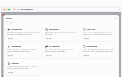
Guardrails
Runtime protection that stops harmful outputs before they reach users
Policies
Define what to govern, when to alert, and how to respond automatically
Control
Complete visibility into your AI systems with real-time monitoring and insights
SUPERWISE Chat: Private AI Workspace
A chatbot experience your team already knows, with guardrails, policies, and audit trails built-in, not bolted on. Your teams need private, safe, compliant AI tools, without the enterprise tax or governance gaps.
Built-in Guardrails
PII detection, toxicity filtering, and jailbreak protection on every interaction.
Complete Audit Trail
Every interaction is attributable and reviewable for regulated workflows.
Business Assistant
Production-ready AI assistant in every tier—doesn’t count toward Customizable Agents.
Model Flexibility
Use any LLM provider with consistent governance across all models.
SUPERWISE AMP
The System Behind the Experience
SUPERWISE AMP is the AI control plane; authority, policy, accountability lives here. Control and trust mean your AI is safe.
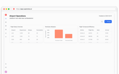
Platform(Control Plane)
Governance across your entire AI environment. Track every model, agent, and decision.
Learn MoreAgent Studio
Design, deploy, and govern AI agents with visual workflows, automated testing, and production-grade controls.
Learn MoreGuardrails
Runtime protection that stops harmful outputs before they reach users. Policy evaluation in under 10ms.
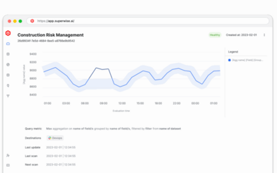
Learn MoreObservability
Supporting signals that inform governance decisions. Know the operational state of your governed AI systems.
Learn MorePolicies
Define what to govern, when to alert, and how to respond. Your governance rules, enforced automatically.
Learn MoreIntegrations
Connect to 50+ LLM providers, vector databases, and enterprise tools in minutes.
Learn MoreCentralized AI Governance = Trusted Results
Deploy AI with confidence. Complete visibility, real-time guardrails, and audit trails for every model and agent.
Free Starter Edition. No credit card required.